Table of Contents
Matrix Product States
Matrix Product States (mps) are an efficient approximation for a general weakly-entangled quantum state. The main idea is to approximate a general quantum state by a sum of simple product states. This sum of product states is generated by a matrix product of $d\cdot n$ matrices, whereby $n$ denotes the number of physical particles (e.g. spin,electrons) with local dimension $d$ (e.g. spinup/spindown). The following introduction to mps follow the review article “The density-matrix renormalization group in the age of matrix product states” by Ulrich Schollwöck1) and the bachelor thesis of Thomas Köhler.
Definition of MPS
In the following we want to focus on a one-dimensional spin-1/2-chain with $L$ sites and open boundaries. On each site there are two (physical) states $\sigma_i=\{\uparrow, \downarrow\}$. Any quantum state that describes the spins on this chain can be expressed by:
\begin{align} \lvert\psi\rangle = \sum_{\sigma_1, \ldots, \sigma_L} c_{\sigma_1\ldots\sigma_L} \lvert {\sigma_1, \ldots, \sigma_L} \rangle \end{align}
The coefficients are $(c_{\sigma_1\ldots\sigma_L} \in {C})$ and their number will increase exponentially $(2^L)$ with the length of the chain. Therefore we cannot represent states for long chains as we cannot represent all coefficients. In MPS every coefficients is given by a matrix product $A_{\sigma_1}\cdot\ldots \cdot A_{\sigma_L}$, whereby each matrix belongs locally to a site (and physical index) and just has a limited number of values.
\begin{align} \lvert\psi\rangle = \sum_{\sigma_1, \ldots, \sigma_L} A^{\sigma_1}\cdot\ldots \cdot A^{\sigma_L} \lvert {\sigma_1, \ldots, \sigma_L} \rangle \end{align}
Construction of MPS from a known quantum state
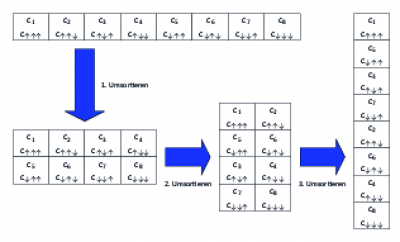
To get an MPS from a known quantum state with coefficients $c_{\sigma_1\ldots\sigma_L}$ we have to shuffle the $2^L$ coefficients into a matrix $c^\prime$ of dimension $2 \times 2^{L-1}$.
\begin{align} c_{\sigma_1\ldots\sigma_L} = c_{\sigma_1, (\sigma_2\ldots\sigma_L)}^\prime \end{align}
Now we will employ a single-value-decomposition2) on the matrix $c^\prime$:
\begin{align} c_{\sigma_1, (\sigma_2\ldots\sigma_L)}^\prime = \sum_{a_1}^{r_1} U_{\sigma_1, a_1} S_{a_1, a_1} (V^\dagger)_{a_1, (\sigma_2\ldots\sigma_L)} \end{align}
Next we generate from $S$ and $V^\dagger$ a new $c_{a_1\sigma_2\ldots\sigma_L}^\prime$, that will be reshuffled into a matrix $c_{(a_1\sigma_2),(\sigma_3\ldots\sigma_L)}^{\prime\prime}$. Furthermore the matrix $U$ (with $U^\dagger U =1$) will be reshuffled into two $A^{\sigma_1}$-matrices, with coefficients: $A^{\sigma_1}_{1,a_1}=U_{\sigma_1,a_1}$. One obtains:
\begin{align} c_{\sigma_1,\ldots\, \sigma_L}=\sum_{a_1}A_{1,a_1}^{\sigma_1}c_{(a_1\sigma_2),(\sigma_3\ldots\sigma_L)}^{\prime\prime} \end{align}
One continues with an svd on $c_{(a_1\sigma_2),(\sigma_3\ldots\sigma_L)}^{\prime\prime}$. The new $S$ and $V^\dagger$ will again be combined and reshuffled into two $A$-matrices. The new coefficients are now: $A^{\sigma_2}_{a_1,a_2} = U_{(a_1\sigma_2), a_2}$. This procedure is repeated until site $L-1$ is reached. One finally obtains:
\begin{align} c_{\sigma_1,\ldots\, \sigma_L} &=\sum_{a_1}\cdots\sum_{a_{l-1}}A_{1,a_1}^{\sigma_1}\cdots A_{a_{l-2},a_{l-1}}^{\sigma_{l-1}}\underbrace{c_{(a_{l-1}\sigma_{l}), (\sigma_{l+1}\ldots\sigma_L)}^{\prime\cdots\prime}}_{M_{a_{L-1},a_L}^{\sigma_L}}\newline &=A^{\sigma_1}\cdots A^{\sigma_{L-1}}M^{\sigma_L} \end{align}
The $A$-matrices fullfill the condition for left-normalization $\sum_{\sigma_l}A^{\sigma_l\dagger}A^{\sigma_l}= 1$. One can also construct a MPS with right-normalized matrices by starting from the left and reshuffling the $V^\dagger$ into $B$-matrices, always continuing with $U$ and $S$. The $B$-matrices will the fullfill the condition for right-normalization: $\sum_{\sigma_l}B^{\sigma_l}B^{\sigma_l\dagger}= 1$. One can also generate a mixed-normalized state by starting from both sides.
Scalar product
The scalar product for two MPS is given by:
\begin{align} \langle \phi \lvert \psi \rangle = \sum_{\boldsymbol{\sigma\sigma^\prime}}\langle \boldsymbol{\sigma^\prime} \lvert \tilde{M}^{\sigma_1^\prime *}\cdots\tilde{M}^{\sigma_L^\prime *}M^{\sigma_1}\cdots M^{\sigma_L}\lvert \boldsymbol{\sigma} \rangle \end{align}
This can be simplified to:
\begin{align} \langle \phi \lvert \psi \rangle = \sum_{\boldsymbol{\sigma}}\tilde{M}^{\sigma_1*}\cdots\tilde{M}^{\sigma_L *}M^{\sigma_1}\cdots M^{\sigma_L} \end{align}
The computation of this expression is computationally very inefficient as one has to calculate $2^L \cdot (2L-1)$ matrix-multiplications. That means that the complexity will increase exponentially with chain length. But we can reformulate the expression, so that we just need $2L$ additions and $4L-2$ matrix-multiplications, which just scales polynomially.
\begin{align} \langle \phi \lvert \psi \rangle &= \sum_{\sigma_L}\tilde{M}^{\sigma_1\dagger}\left(\cdots\left(\sum_{\sigma_2}\tilde{M}^{\sigma_2\dagger}\left(\sum_{\sigma_1}\tilde{M}^{\sigma_1\dagger}M^{\sigma_1}\right)M^{\sigma_2}\right)\cdots\right) M^{\sigma_L} \end{align}
Matrix-Product-Operator (MPO)
Analogously to quantum states, we can also express the operators as Matrix-Product-operators. We simply define:
\begin{align} \hat O & = \sum_{\boldsymbol{\sigma}, \boldsymbol{\sigma^{\prime}}} c_{(\sigma_1\ldots\sigma_L)(\sigma_1^{\prime}\ldots\sigma_L^{\prime})} \lvert {\boldsymbol{\sigma}} \rangle \langle {\boldsymbol{\sigma'}} \lvert \newline & = \sum_{\boldsymbol{\sigma}, \boldsymbol{\sigma^{\prime}}} c_{(\sigma_1\sigma_1^{\prime})\ldots(\sigma_L\sigma_L^{\prime})} \lvert {\boldsymbol{\sigma}} \rangle \langle {\boldsymbol{\sigma^{\prime}}} \lvert \newline & = \sum_{\boldsymbol{\sigma}, \boldsymbol{\sigma^{\prime}}} W^{\sigma_1\sigma_1^{\prime}}\ldots W^{\sigma_L\sigma_L^{\prime}} \lvert {\boldsymbol{\sigma}} \rangle \langle {\boldsymbol{\sigma^{\prime}}} \lvert \end{align}
The $W$-matrices will do the same job as the $M$-matrices of MPS. The difference is that they have two physical indices.
Application of a MPO
The application of a MPO on a MPS is expressed by:
\begin{align} \hat O \lvert \psi \rangle & = \sum_{\boldsymbol{\sigma}, \boldsymbol{\sigma^{\prime}}, \boldsymbol{\sigma^{\prime\prime}}} (W^{\sigma_1\sigma_1^{\prime}}\ldots W^{\sigma_L\sigma_L^{\prime}})(M^{\sigma_1^{\prime\prime}}\cdots M^{\sigma_L^{\prime\prime}})\lvert {\boldsymbol{\sigma}} \rangle \underbrace{\langle {\boldsymbol{\sigma^\prime}} \lvert {\boldsymbol{\sigma^{\prime\prime}}} \rangle}_{\delta_{\sigma^{\prime}\sigma^{\prime\prime}}}\newline & = \sum_{\boldsymbol{\sigma}, \boldsymbol{\sigma^{\prime}}} (W^{\sigma_1\sigma_1^{\prime}}\ldots W^{\sigma_L\sigma_L^{\prime}})(M^{\sigma_1^{\prime}}\cdots M^{\sigma_L^{\prime}})\lvert {\boldsymbol{\sigma}} \rangle \newline & = \sum_{\boldsymbol{\sigma}} \tilde{M}^{\sigma_1}\cdots \tilde{M}^{\sigma_L} \lvert\boldsymbol{\sigma}\rangle = \lvert \tilde\psi\rangle \end{align}
The values of the $\tilde{M}$ matrices are given by:
\begin{align} \tilde{M}^{\sigma_i} = \sum_{\sigma_i^{\prime}}W^{\sigma_i\sigma_i^{\prime}}_{b_{i-1},b_i}M^{\sigma_i^{\prime}}_{a_{i-1}, a_i} \end{align}
$\lvert\tilde\psi\rangle$ is a therefore a new MPS, but with a larger dimension. So an expectation value of an operator can be calculated by
\begin{align} \langle \psi \lvert \hat O \lvert \psi \rangle = \langle \psi \lvert \tilde \psi \rangle \end{align}
Repeated application of an operator onto a state therefore increases strongly the dimension of the state.
Hamilton-Operator
A general Hamilton-operator such as:
\begin{align} \hat H = \sum_{i=1}^{L-1}\frac{J}{2}\hat S_i^+\hat S_{i+1}^- + \frac{J}{2}\hat S_i^-\hat S_{i+1}^+ + J^z\hat S_i^z\hat S_{i+1}^z-h_z\sum_i^L \hat S_i^z-h_x\sum_i^L \hat S_i^x \end{align}
can be constructed analytically as an MPO. This is reasoned in the special Tensor-Product-structure of the Hamiltonian:
\begin{align} \hat H = J^z\hat S_1^z\otimes\hat S_2^z\otimes\hat I_3\otimes\hat I_4\ldots + \hat I_1\otimes J^z\hat S_2^z\otimes\hat S_3^z\otimes\hat I_4\ldots+\ldots \end{align}
To construct the Hamiltonian we have to give the matrices.
\begin{align} \hat W^{\left[i\right]}=\sum_{\sigma_i, \sigma^\prime_i}W^{\sigma_i\sigma_i^\prime}\lvert\sigma_i\rangle\langle\sigma_i^{\prime}\lvert \end{align}
They are given by:
\begin{align} \hat W^{\left[i\right]} = \begin{bmatrix} \hat I & 0 & 0 & 0 & 0 \newline \hat S^+ & 0 & 0 & 0 & 0 \newline \hat S^- & 0 & 0 & 0 & 0 \newline \hat S^z & 0 & 0 & 0 & 0 \newline -h_z\hat S^z-h_x\hat S^x & (J/2)\hat S^- & (J/2)\hat S^+ & J^z\hat S^z & \hat I \end{bmatrix} \end{align}
With the special first and last matrices:
\begin{align} \hat W^{\left[1\right]} &= \begin{bmatrix} -h_z\hat S^z-h_x\hat S^x & (J/2)\hat S^- & (J/2)\hat S^+ & J^z\hat S^z & \hat I \end{bmatrix}\\ \hat W^{\left[L\right]} &=\begin{bmatrix} \hat I\newline \hat S^+ \newline \hat S^- \newline \hat S^z\newline -h_z\hat S^z-h_x\hat S^x \end{bmatrix} \end{align}
The $W^{\sigma_i,\sigma_i^\prime}$ can be directly constructed from the physical operators:
\begin{align} \hat W^{\sigma_i\sigma_i^{\prime}}_{j, k} = \langle\sigma_i\lvert\hat W^{\left[i\right]}_{j, k} \lvert\sigma_i'\rangle \end{align}
©: This site was created by Piet Dargel and Thomas Köhler


