Table of Contents
Examples / test cases
In this chapter we will present some examples for the applet and compare them with analytical solutions. You can easily reproduce the simulations just by clicking on the link and the applet will be started with these values.
Ising-Model (without magnetic field)
The Ising-model, named after Ernst Ising - is a theoretical model for the description of ferro and antiferromagnetism. It simply consists of spins on a chain (lattice in higher dimensions) that interact just with their neighbours. For an introduction see Ref. 1) or 2).
In the isotropic case - that means without a magnetic field - there is no phase transition in one dimension as known from the exact solution.3). In two dimension there are phase transitions Im zweidimensionalen Fall existieren dahingegen Phasenübergänge as the exact solution shows 4) 5). For higher dimensions there are no exact solutions, but there are proofs for the existence of phase transitions. 6).
The Hamiltonian \(\hat H\) of the Ising-model without magnetic field with constant nearest neighbour interaction and open boundary conditions is given by \begin{equation*} \hat H= J^z\sum_{i=1}^{N-1}\hat S_i^z \hat S_{i+1}^z \end{equation*} The groundstate energy for a chain with N sites is given by: \begin{equation*} E_0 = -\frac{(N-1)\cdot \lvert J^z\lvert}{4} \end{equation*} You can test this model as an example for a chain with 8 sites here. You will find a groundstate energy of \begin{equation*} E_0 = -\frac{(8-1)\cdot \lvert J^z\lvert}{4}=-1.75 \end{equation*}
Antiferromagnetism
For \(J>0\) the system will be anti-ferromagnetic. That means that all the spins align anti-parallel. \begin{equation*} \lvert\psi\rangle = \lvert\uparrow\downarrow\uparrow\ldots\rangle \quad \text{or} \quad \lvert\psi\rangle = \lvert\downarrow\uparrow\downarrow\ldots\rangle \end{equation*} This state is called the Néelstate. The groundstate can be any superposition of these two states - it is twofold degenerated. The DMRG will converge randomly in one of these two states. It can also happen that the states change while sweeping. In order to control the convergence into one of these states one has to implement good quantum numbers into the algorithm. Then one can lift the degeneracy by calculating in a certain \(S_z\)-sector (for chains with an odd number of sites).
The expectation value of \(\hat S_i^z\) at site \(i\) is given by: \begin{equation*} \langle\hat S_i^z\rangle=\pm \frac{1}{2} \end{equation*} The expectation value for the total magnetization \(\hat S^z\) is given by: \begin{equation*} \langle\hat S^z\rangle=\left\{\begin{array}{cl} 0, & \text{if }N \text{ even}\newline \pm \frac{1}{2}, & \text{if }N \text{ odd} \end{array}\right. \end{equation*} You can test this for a chain with an even number of sites here und for a chain with an odd number of sites here.
Ferromagnetism
For \(J<0\) the system is ferromagnetic. The all spins will be aligned parallel in the groundstate: \begin{equation*} \lvert\psi\rangle = \lvert\uparrow\uparrow\uparrow\ldots\rangle \quad \text{or} \quad \lvert\psi\rangle = \lvert\downarrow\downarrow\downarrow\ldots\rangle \end{equation*} The groundstate is again two-fold degenerated and can be any superposition of these two states. The DMRG will again randomly converge to one of these states. The expectation value of \(\hat S_i^z\) will be the same for all spins and therefore the expectation value for \(\hat S^z\) will be given by: \begin{equation*} \langle\hat S^z\rangle=\pm \frac{N}{2} \end{equation*} You can test the ferromagnetic system here.
Ising-Model (with longitudinal magnetic field)
The Hamiltonian \(\hat H\) for the Ising model with longitudinal magnetic field in z-direction is given by: \begin{equation*} \hat H= J^z\sum_{i}\hat S_i^z \hat S_{i+1}^z + h^z\hat S_i^z \end{equation*} Hereby \(h^z\) denotes the magentic field. %In the following we will use \(h^z\ll J^z\). The antiferromagnet shows a phase transition at \(T=0\) to a ferromagnetic state at magnetic field \(h^z_c = J^z\). There is no phase transition for the ferromagnetic system.
Antiferromagnet
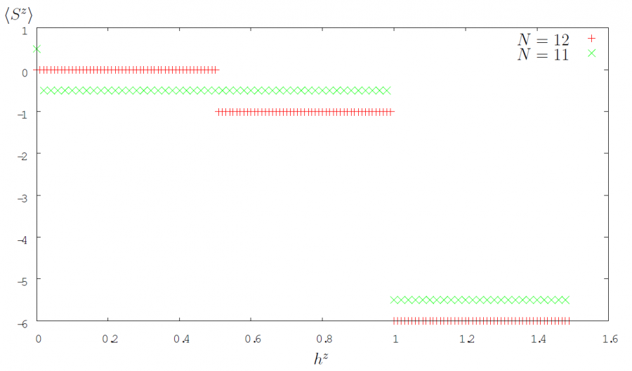
If \(h^z\ll J^z\), the the sign of \(h^z\) will give the direction of the spins at the end of the chain with an odd number of sites in the antiferromagnetic system: \begin{equation*} \lvert\psi\rangle=\left\{\begin{array}{cl} \lvert\uparrow\downarrow\uparrow\cdots\downarrow\uparrow\rangle, & \text{if }h^z < 0\newline \lvert\downarrow\uparrow\downarrow\cdots\uparrow\downarrow\rangle, & \text{if }h^z>0 \end{array}\right. \end{equation*} You can simulate this system here for positve \(h^z\) and here for negative \(h^z\).
For a chain with an even number of sites the groundstate energy is given by:
\begin{equation*}
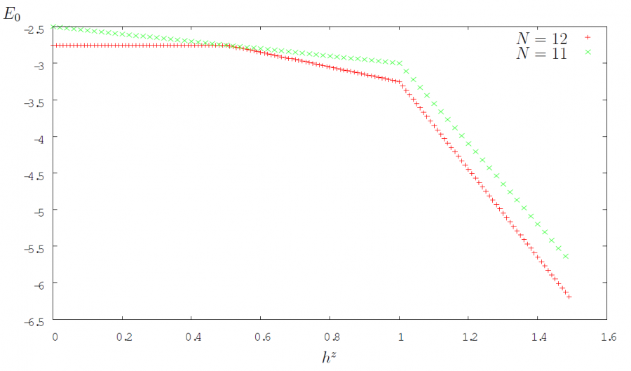
E_0=\left\{\begin{array}{cl} -\frac{N-1}{4}\lvert J^z\lvert, & \text{if }h^z \leq \frac{J^z}{2} \text{, Antiferromagnet: }\lvert\uparrow\downarrow\uparrow\cdots\uparrow\downarrow\rangle \newline -\frac{N-3}{4}\lvert J^z\lvert - \lvert h^z\lvert, & \text{if }\frac{J^z}{2}< h^z\leq J^z \text{, defect Antiferromagnet: }\lvert\uparrow\downarrow\uparrow\cdots\uparrow\uparrow\rangle\newline \frac{N-1}{4}\lvert J^z\lvert - \frac{N}{2}\lvert h^z\lvert, & \text{if }J^z< h^z \text{, Ferromagnet: }\lvert\uparrow\uparrow\uparrow\cdots\uparrow\uparrow\rangle\end{array}\right.
\end{equation*}
For a chain with an odd number of sites the groundstate energy is given by:
\begin{equation*}
E_0=\left\{\begin{array}{cl} -\frac{N-1}{4}\lvert J^z\lvert - \frac{\lvert h^z\lvert}{2}, & \text{if } h^z\leq J^z \text{, Antiferromagnet: }\lvert\uparrow\downarrow\uparrow\cdots\uparrow\rangle\newline \frac{N-1}{4}\lvert J^z\lvert - \frac{N}{2}\lvert h^z\lvert, & \text{if }J^z< h^z \text{, Ferromagnet: }\lvert\uparrow\uparrow\uparrow\cdots\uparrow\uparrow\rangle\end{array}\right.
\end{equation*}
The form of the groundstate energy will change when the external magnetic field \(h^z \leq h^z_c\) is larger than the antiferromagnetic interaction and it is energetically cheaper for the system to align in direction of the magnetic field. The special intermediate case is just reasoned in the open boundary conditions as the spins at the end of the chain will align in the direction of the magnetic field before the inner spins (for a chain with an even number of sites). You can easily identify the three sectors in the following figure:
[ ]
[
]
[ ]
]
Ferromagnetism
The sign of the external magnetic field \(h^z\) gives the direction of the spins. \begin{equation*} \lvert\psi\rangle=\left\{\begin{array}{cl} \lvert\uparrow\uparrow\uparrow\rangle, & \text{if }h^z < 0\newline \lvert\downarrow\downarrow\downarrow\rangle, & \text{if}h^z>0 \end{array}\right. \end{equation*} The expectation value of \(S^z\) is also given by \(h^z\). \begin{equation*} \langle\psi\lvert\hat S^z\lvert\psi\rangle=\left\{\begin{array}{cl} \frac{N}{2}, & \text{if }h^z < 0\newline -\frac{N}{2}, & \text{if }h^z>0 \end{array}\right . \end{equation*} The groundstate energy is given by \begin{equation*} E_0 = -\frac{(N-1)\cdot \lvert J\lvert}{4} - \lvert h^z \lvert\frac{N}{2} \end{equation*}
Ising-Model (with transverse magnetic field)
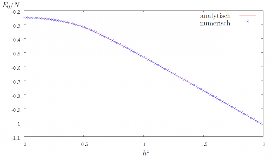
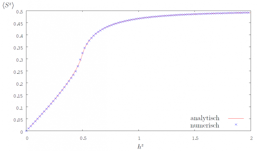
The Hamiltonian of the Ising model in the transverse magnetic field is given by: \begin{equation*} \hat H= J^x\sum_{i}\hat S_i^x \hat S_{i+1}^x + h^z\hat S_i^z \end{equation*} The system was solved exactly 7) and shows a phasetransition for \(h^z = J^x/2\). In order to show this phase transition one has to do a finite-size-scaling. We calculated \(E_0/N\), \(\langle S^x\rangle/N\) and \(\langle S^z\rangle/N\) for different system sizes N and plot them vs. \(1/N\) for different \(h^z\). Then using linear regression one can determine the values \(E_0(h^z)\), \(\langle S^x\rangle (h^z)\) and \(\langle S^x\rangle (h^z)\) for the infinite system. The analytical solution 8) give for the groundstate energy and the expectation value of \(S^z\) depending on \(\lambda=J/2h^z\): \begin{equation*} \frac{E_0}{J^xN}(\lambda)=\frac{2}{\pi}(1+\lambda)E\left(\frac{\pi}{2}, \Theta\right) \end{equation*} Hereby \(\Theta^2=\frac{4\lambda}{(1+\lambda)^2}\) and \(E\left(\frac{\pi}{2}, \Theta\right)\) are elliptical integrals of the second kind. \begin{equation*} \langle \hat S^z \rangle (\lambda) = \frac{1}{2}G(0, \lambda)\quad\text{with }G(n,\lambda )=L(n,\lambda )+\lambda L(n+1,\lambda ) \end{equation*} Using \(G(n,\lambda )=L(n,\lambda )+\lambda L(n+1,\lambda )\) and \begin{equation*} L(n,\lambda )=1/\pi \int_0^\pi dk \Lambda_k^{-1}cos(k n) \end{equation*} with \(\Lambda_k^2=1+\lambda^2+ \lambda \cos(k)\) proportional to an elliptical integral of first kind. In the figures we show the results of the MPS-simulation with finite-size-scaling and the analytical solution.
Heisenberg-Model
Within the Heisenberg-model the spins are not limited to specific direction anymore. They can point in any of the three space directions. The Hamiltonian of the Heisenberg-chain in one dimension is therefore given by:
\begin{equation*} \hat H = J\sum_i \left(\hat S^x_i \hat S^x_{i+1} + \hat S^y_i \hat S^y_{i+1} + \hat S^z_i\hat S^z_{i+1}\right) \end{equation*}
The ntiferromagnetic Heisenberg-model is much more difficult to solve in comparison to the Ising model as it is also without magnetic field a quantummechanical model. This is reasoned in the non-commuting operators \(S^x\),\(S^y\),\(S^z\). But in one dimension there is a solution via the Bethe-Ansatz (For an introduction see Ref. 9).
You can test the antiferromagnetic system here. The Bethe-Ansatz for the periodic system gives a groundstate energy per bond of \(\frac{1}{4}-ln(2)=-0.443147\). Using finite size scaling for the open boundary system the fit for the groundstate energy gives \(-0.4407\pm0.00057\).
©: This site was created by Piet Dargel and Thomas Köhler


